Encapsulation theory: the isoledensal configuration efficiency limit.

Edmund Kirwan^*

www.EdmundKirwan.com

Abstract

This paper shows how the maximum possible isoledensal configuration efficiency of an indefinitely large software system is constrained by the number of program units per subsystem. It is then shown how the configuration efficiency of an indefinitely large software system depends on the ratio of the total number of information-hiding violational software units divided by the total number of program units.

Keywords

Encapsulation, potential coupling, configuration efficiency.

1. Introduction

The isoledensal configuration efficiency of a software system was introduced in [1] and defined as being that proportion of potential coupling that a system expresses over and above the minimum isoledensal potential coupling of that system.

Two questions in [1] concerning this configuration efficiency, however, remained unanswered.

The first relates to figure 24 in the referenced paper, reproduced here:

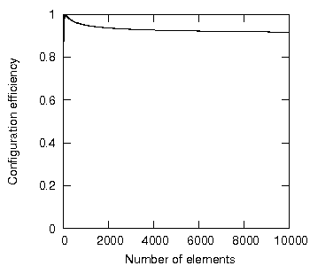
Figure 24: Configuration efficiency with ten program units per subsystem

What is the precise relationship between the configuration efficiency and the constraint of a fixed number of program units per subsystem, as show in figure above?

The second question relates to table 2 in the referenced paper, reproduced here:

	Num. elements	Potential coupling	I.C.E.	I.H.V.
SEdit	135	16956	0.09	93%
Fractality	240	19042	0.86	25%
HSQLdb	283	61633	0.37	72%
Jasper Reports	316	99540	0	100%
JBPM	366	133590	0	100%
Manta- Ray	384	132298	0.12	89%
Blue Marine	468	194991	0.13	89%
Jboss	4244	17619836	0.02	98%
Eclipse	39114	933916300	0.4	61%

Table 2: Sample systems and associated metrics

Why, in table 2, is there a correlation between the isoledensal configuration efficiency (I.C.E.) and the ratio of the number of public program units divided by the total number of program units (the I.H.V., expressed as a percentage)? (Recall that the public accessor in Java – in which all the systems above were written – is the means of implementing the more general notion of information-hiding violation.)

This paper answers both of these questions.

Note that this paper covers only the non-hierarchical encapsulation context.

2. Fixed-sized subsystems

As software systems grow, the number of program units per subsystem must also grow if the system's potential coupling is to be minimised and the configuration efficiency maximised. For example, a system of 10,000 program units, with one information-hiding violation per subsystem, would require one hundred program units in each subsystem.

Modern software practices, however, tend to restrict the number of program units per subsystem to a figure much lower than 100. No figure is universally agreed upon, but subsystems typically contain fewer than fifty program units.

The question may then be asked: if a programmer restricts the number of program units per subsystem, how does this affect the potential coupling expressed by the system? Is there a precise relationship between a fixed upper limit to the number of program units per subsystem and the maximum possible configuration efficiency of a system?

The answer to this last question is yes.

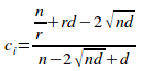
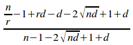
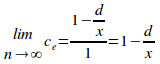
If a programmer restricts the number of program units per subsystem to x, say, and if d is the specific information-hiding violation (the number of public program units per subsystem) then the maximum possible configuration efficiency of that system as it grows indefinitely large is given by the equation (see proposition 2.3):

This maximum possible configuration efficiency of an indefinitely large system as is called the configuration efficiency limit.

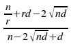
Thus in the system discussed above, if the programmer restricts the number of program units per subsystem to fifty and with each subsystem containing one public program unit, then the configuration efficiency limit of that system is:

If the programmer restricts the same system to 10 program units per subsystem, the configuration efficiency limit will be 0.9, as suggested by figure 24, shown in the introduction.

2. System information hiding.

Examining the data in table 2, we see that Jboss, for example, has a configuration efficiency of 0.02 and the number of public classes expressed as a percentage of the total number of classes is 98%. Expressing this percentage as a ratio, we see that Jboss's public-to-total class ratio is 0.98, which seems to be one minus the configuration efficiency. Eclipse, similarly, as a configuration efficiency of 0.4 and a ratio of 0.61, again, approximately one minus the configuration efficiency.

The question may then be asked: is there a precise relationship between the maximum possible configuration efficiency of a system and the ratio of the number of violational program units divided by the total number of program units?

The answer is yes.

If the total number of a program units in a system is n and the total number of information hiding violational program units is |p(G)| then the configuration efficiency limit can also be expressed as (see proposition 2.4):

The ratio in this equation is the ratio of the number of public classes divided by the total number of classes in a system. This equation only holds for large systems, which is why table data correlate more strongly for the larger than the smaller systems. This also presents a method for calculating a convenient approximation to the configuration efficiency for large systems.

3. Conclusions

This paper suggests both that the modern practice of constraining packages sizes is a viable mechanism for managing the potential coupling of indefinitely large systems, and that the maximum possible configuration efficiency of indefinitely large systems is related to the total number of violational program units.

Appendix A

Proposition 2.1.

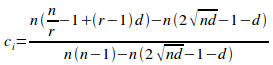
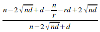
Given a uniformly distributed encapsulated set G of n elements and of r disjoint primary sets, with each disjoint primary set having an information-hiding violation of d, the isoledensal configuration inefficiency c_i is given by the equation:

Proof:

From section 6.5.4. of [1], the isoledensal configuration inefficiency is given by:

(i)

Where:

= actual system potential coupling

= minimum system isoledensal potential coupling

= maximum system potential coupling

From proposition 1.1 of [1]:

From proposition1.8 of [1]:

From proposition 1.14 of [1]:

Substituting all three equations into (i) gives:

=

=

=

QED

Proposition 2.2.

Given a uniformly distributed encapsulated set of n elements and of r disjoint primary sets, with each disjoint primary set having an information-hiding violation of d, the isoledensal configuration efficiency c_e is given by the equation:

(i)

Proof:

From section 6.5.4. of [1], the isoledensal configuration efficiency is given by:

c_e = 1 - c_i

From proposition 2.1:

c_i =

Substituting into (i) gives:

c_e = 1 -

=

=

=

QED

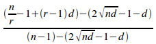
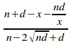
Proposition 2.3.

Given a uniformly distributed encapsulated set of n elements and of r disjoint primary sets, with each disjoint primary set having an information-hiding violation of d, and given that the i^th disjoint primary set K_i contains the fixed number x elements, the limit of the isoledensal configuration efficiency as the set grows indefinitely large is given by:

Proof:

From proposition 2.2:

c_e = (i)

By definition:

and so

Substituting both of these equations into (i) gives:

c_e =

=

=

Taking the limit as n tends to infinity gives:

QED

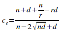
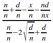
Proposition 2.4

Given a uniformly distributed encapsulated set G of n elements and of r disjoint primary sets, with each disjoint primary set having an information-hiding violation of d, and given that G has an information-hiding violation set of V, the limit of the isoledensal configuration efficiency as the set grows indefinitely large is given by:

Proof:

From proposition 2.3, where the i^th disjoint primary set K_i contains the fixed number x elements, the limit of the isoledensal configuration efficiency of G as the set grows indefinitely large is given by:

(i)

By definition:

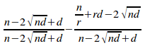
Substituting this into (i) gives:

(ii)

But by item (iii) of definition [D1.14] in [1]:

Substituting this into (ii) gives:

QED

References

[1] "Encapsulation theory fundamentals," Ed Kirwan, www.EdmundKirwan.com/pub/paper1.pdf

[2] "Encapsulation theory: the isoledensal configuration efficiency limit," Ed Kirwan, www.EdmundKirwan.com/pub/paper2.pdf